Advanced Slurm

This lesson expands on the principles of Slurm job configuration and parallelization from the first Slurm lesson. It introduces Slurm job dependencies, pipeline management techniques, and environment management and sharing with Conda.

Lesson Setup

For this lesson, you will need to connect to a Talapas login node through a shell application of your choice.

For convenience, we recommend the Talapas OnDemand shell.

Make sure you are in your home directory.

cd ~

Copy the slurm_day2 folder to your home directory. As always, make sure to use the -r flag to recursively copy the folder’s contents.

cp -r /projects/racs_training/intro-hpc-f25/slurm_day2/  .

Navigate inside the slurm_day2 directory you copied over.

cd slurm_day2

Evaluating Resource Usage on Running Jobs with htop

Remember the seff command? That’s a great way to evaluate resource usage of a finished job. But what about resource usage for running jobs?

Navigate to the python_pi_example directory and inspect the contents.

cd python_pi_example
ls

calculate_pi.py  calculate_pi.sbatch

Inspect calculate_pi.sbatch.

cat calculate_pi.sbatch

#!/bin/bash

#SBATCH --partition=preempt              ### Partition (like a queue in PBS)
#SBATCH --account=racs_training          ### Account used for job submission

### NOTE: %u=userID, %x=jobName, %N=nodeID, %j=jobID, %A=arrayMain, %a=arraySub
#SBATCH --job-name=digits_of_pi          ### Job Name
#SBATCH --output=%x.log                  ### File in which to store job output

#SBATCH --time=0-00:60:00                ### Wall clock time limit in Days-HH:MM:SS
#SBATCH --nodes=1                        ### Number of nodes needed for the job
#SBATCH --mem=100M                       ### Total Memory for job in MB -- can do K/M/G/T for KB/MB/GB/TB
#SBATCH --cpus-per-task=1                ### Number of cpus/cores to be launched per Task

### Load needed modules
module purge
module load python3/3.11.4

### Run your actual program
srun -u python3 -u calculate_pi.py 30000

This is a serial job that loads the python3 module and executes a Python script that computes the first 30000 digits of pi. Observe that this job runs on the preempt partition. Both error and output logs are written to a single digits_of_pi.log, which (if there are no errors) will contain pi approximated to the first 30000 digits.

Use cat to inspect calculate_pi.py.

This script takes in an integer argument num_digits from the command line, then calculates that many of pi.

cat calculate_pi.py

#!/usr/bin/env python3

import sys

def calcPi(limit):  # Generator function
    """
    Prints out the digits of PI
    until it reaches the given limit
    """

    q, r, t, k, n, l = 1, 0, 1, 1, 3, 3

    decimal = limit
    counter = 0

    while counter != decimal + 1:
            if 4 * q + r - t < n * t:
                    # yield digit
                    yield n
                    # insert period after first digit
                    if counter == 0:
                            yield '.'
                    # end
                    if decimal == counter:
                            break
                    counter += 1
                    nr = 10 * (r - n * t)
                    n = ((10 * (3 * q + r)) // t) - 10 * n
                    q *= 10
                    r = nr
            else:
                    nr = (2 * q + r) * l
                    nn = (q * (7 * k) + 2 + (r * l)) // (t * l)
                    q *= k
                    t *= l
                    l += 2
                    k += 1
                    n = nn
                    r = nr


def main():  # Wrapper function

    num_digits = sys.argv[1]

    for d in calcPi(int(num_digits)):
        print(d, end='')

if __name__ == '__main__':
    main()

For those of you unfamiliar with Python, this is a single-threaded algorithm that uses a loop to return successive digits from a generator function, calc_pi.

Launch the Slurm job with sbatch.

sbatch calculate_pi.sbatch

Submitted batch job 39549813

Check your queue. Note the node number (hostname) of the compute node where the job is currently running.

squeue --me

             JOBID PARTITION     NAME     USER ST       TIME  NODES NODELIST(REASON)
          39549813   preempt digits_o    emwin  R       0:06      1 n0105

As we can see, we are currently running on node n0105.

Because we have an active Slurm task on node n0105, we can remote into that compute node from the login node with ssh.

ssh n0105

Enter the password to your DuckID when prompted. Confirm that you are connected with the hostname command.

hostname

n0105.talapas.uoregon.edu

While you are on the compute node, the htop command can be used to evaluate the resources usage of your running processes.

htop -u $USER

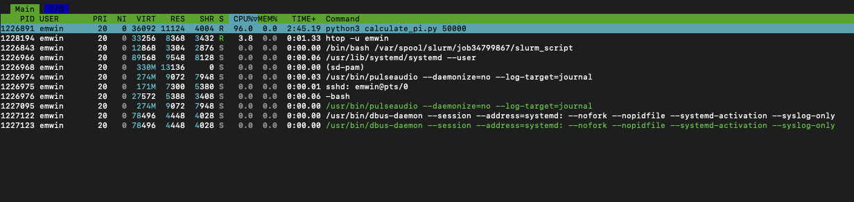
• The USER column is the DuckID of the user who launched the process.
• The RES column measures RAM per process in KB.
• The CPU% column measures the percentage of CPU time used by the process. 100% indicates full usage of a single CPU core.
• The MEM% column indicates the percentage of memory the process is using.
• The TIME column indicates how long the process has been running in seconds.

From this, we can see that the calculate_pi script uses the single core it has been allocated very effeciently (97.5%) but uses almost no RAM. This is by design, as Python generators are more memory effecient than lists or sequences.

Your connection to the compute node will terminate when your job terminates. After the job has finished, you can use seff to get more granular information about your job.

Let’s use sacct to get more information about the finished job.

sacct --units=M --format=JobId,JobName,ReqMem,MaxRss,ReqCPUs,AllocCPUs,Elapsed,State

JobID           JobName     ReqMem     MaxRSS  ReqCPUS  AllocCPUS    Elapsed      State 
------------ ---------- ---------- ---------- -------- ---------- ---------- ---------- 
39549813     digits_of+       100M                   1          1   00:01:03  COMPLETED 
39549813.ba+      batch                 4.64M        1          1   00:01:03  COMPLETED 
39549813.ex+     extern                 0.12M        1          1   00:01:04  COMPLETED 
39549813.0      python3                 5.68M        1          1   00:01:01  COMPLETED 

If you’ve run several jobs recently, you can pass in a special flag to sacct to indicate that you only want to results from jobs started in the last hour.

sacct --units=M --format=JobId,JobName,ReqMem,MaxRss,ReqCPUs,AllocCPUs,Elapsed,State -S now-1hour

Finally, let’s confirm the job ran correctly by checking the output log. As the output is quite long, use cut to peek at the first six characters of the output log.

cat digits_of_pi.log | cut -c1-6

3.1415

Now, let’s confirm that there are 30000 digits using the wc -c command to count the characters in the output file.

cat digits_of_pi.log | wc -c

30002

Because the 30000 digits are prefixed with 3., 30002 is the number of characters of output we would expect.

Evaluating Finished Job Resource Usage with seff

Examine this job’s effeciency with seff. Remember to pass in your job id in place of the example.

seff 39549813

Job ID: 39549813
Cluster: talapas
User/Group: emwin/uoregon
State: COMPLETED (exit code 0)
Cores: 1
CPU Utilized: 00:01:01
CPU Efficiency: 96.83% of 00:01:03 core-walltime
Job Wall-clock time: 00:01:03
Memory Utilized: 5.68 MB
Memory Efficiency: 5.68% of 100.00 MB

What does seff tell us here? Our toy job uses the CPU very effeciently, but it uses only 5.68% of the 100MB of RAM requested.

While 100MB is a trivial amount of memory, if you observe your own Slurm job has such low memory effeciency, it will schedule faster and finish just as quickly if you request less memory in future.

For example, requesting 100GB of RAM when your job only requires 8GB is poor Talapas etiquette.

Slurm Job Constraints: Additional CPU Cores

Remember those #SBATCH arugments at the top of each Slurm batch script?

You can override those arguments manually when launching a batch script by passing in the argument followed by the replacement value.

We will use this technique to manipulate certain parameters to see how they affect the performance of the calculate_pi.sbatch. This is faster than manually adjusting parameters in a command line text editor like nano or vim.

When writing and executing Slurm jobs in the context of scientific computing, especially for code used to generate results, it is essential that your batch scripts reflect exactly how your Slurm jobs were executed. We do not recommend overriding batch script arguments through the command line outside the context of development or testing.

First, let’s see if requesting more CPU cores will make the calculate_pi script finish faster.

sbatch --job-name=digits_of_pi_4cpus --cpus-per-task=4 calculate_pi.sbatch 

Submitted batch job 39560052

Because these arguments overwrite what you have in your script, this will launch a job that is identical to our previous iteration except that… 1) it will be named digits_of_pi_4cpus 2) it will request 4 CPU cores rather than 1

How much faster than will this job run? Wait for the job to finish, then use sacct to check the time that job took in the Elapsed column.

sacct --units=M --format=JobId,JobName,ReqMem,MaxRss,ReqCPUs,AllocCPUs,Elapsed,State

JobID           JobName     ReqMem     MaxRSS  ReqCPUS  AllocCPUS    Elapsed      State 
------------ ---------- ---------- ---------- -------- ---------- ---------- ---------- 
39549813     digits_of+       100M                   1          1   00:01:03  COMPLETED 
39549813.ba+      batch                 4.64M        1          1   00:01:03  COMPLETED 
39549813.ex+     extern                 0.12M        1          1   00:01:04  COMPLETED 
39549813.0      python3                 5.68M        1          1   00:01:01  COMPLETED 
39560052     digits_of+       100M                   4          4   00:01:01  COMPLETED 
39560052.ba+      batch                 4.64M        4          4   00:01:01  COMPLETED 
39560052.ex+     extern                 0.05M        4          4   00:01:01  COMPLETED 
39560052.0      python3                 5.91M        4          4   00:00:59  COMPLETED 

While your time may vary, my first job completed in 1:03 and this job completed in 1:01. As you can see, the job that was allocated 4 CPUs rather than 1, did not run 4 times as fast. What happened?

Let’s look more closely at the digits_of_pi_4cpus job with seff.

seff 39560052

Job ID: 39560052
Cluster: talapas
User/Group: emwin/uoregon
State: COMPLETED (exit code 0)
Nodes: 1
Cores per node: 4
CPU Utilized: 00:01:03
CPU Efficiency: 25.82% of 00:04:04 core-walltime
Job Wall-clock time: 00:01:01
Memory Utilized: 5.91 MB
Memory Efficiency: 5.91% of 100.00 MB

Through Slurm allocated 4 cores, the script compute_pi.py does not distribute work among the additional cores because the code is not designed to take advantage of them. It always computes digits one at a time using a single CPU core; it is not parallelized. The job’s CPU-effeciency goes from 97.5% to 23.85% because it only uses one of the four cores.

This isn’t to dismiss the power of parallel computing. Additional CPU cores make jobs that leverage them complete much faster! You will get to see examples of parallelized Python code later in this lesson.

Node Features: Helper Scripts From RACS

Need to decide which nodes (and which partitions) are appropriate for your jobs? RACS has a script that shows available CPU and RAM on each node.

/packages/racs/bin/slurm-show-cpu-mem

This script shows the name of the node, the number of CPU cores on the node, and the amount of RAM (in MB) in that order for each node on Talapas.

...
n0187 128 515048
n0188 128 515048
n0189 128 515048
n0190 128 515048
n0191 128 515048
n0192 128 515048
n0193 128 515048
...

Nodes on the compute partition typically have 128 CPU cores and 500GB of RAM.

To check which partition a node belongs to, find its name in the output of the sinfo command. Let’s look at n0191, a compute node.

sinfo

As you can see, n0191 is one of the nodes in the compute partition.

compute              up 1-00:00:00      1   plnd n0195
compute              up 1-00:00:00      6  drain n[0112-0117]
compute              up 1-00:00:00     35    mix n[0111,0118-0135,0180-0194,0196]

You may also want to know what hardware is associated with each node.

/packages/racs/bin/slurm-show-features

This script shows the node name, processor type, processor architecture, and GPU parameters for each node.

...
n0191 amd,milan,7713
n0192 amd,milan,7713
n0193 amd,milan,7713
n0194 amd,milan,7713
n0195 amd,milan,7713
n0196 amd,milan,7713
n0197 intel,sapphirerapids,6448y,mem-1tb,l40s,gpu-48gb
...

Let’s inspect n0191 again. As you can see, it has an AMD processor and no GPU.

Nodes with extra RAM are indicated with mem-[amount] tags.

n0372 intel,broadwell,e7-4830,mem-1t
n0373 intel,broadwell,e7-4830,mem-1tb
n0374 intel,broadwell,e7-4830,mem-4tb

Nodes with GPUs are also indicated in this list.

n0149 amd,milan,7413,a100,gpu-10gb
n0150 amd,milan,7413,a100,gpu-40gb
n0151 amd,milan,7413,a100,gpu-10gb
n0152 amd,milan,7413,a100,3xgpu-80gb,no-mig

These comma-separated traits are called features.

We can use constraints to direct Slurm to schedule jobs on nodes with specific features (extra RAM, GPU, CPU architecture) based on code hardware requirements.

Using Slurm Job Constraints: Requesting Specific Hardware

Does running a job on different hardware affect performance? For example, do processors with newer architecture perform better than older ones?

Broadwell processors, launched in 2014, are the oldest Intel CPUs available on Talapas. Intel launched its Sapphire Rapids processors in 2023. Processors with this architecture are the newest Intel processors on Talapas.

Let’s return to our calculate_pi job. We know its performance is heavily CPU-dependent from our previous experimentation.

We can use the --constraint parameter to restrict our job to nodes with specific features. In this cause, we want this job to run on a node with a Sapphire Rapids processor.

sbatch --job-name=sapphirerapids_pi --constraint=sapphirerapids calculate_pi.sbatch

Submitted batch job 39570110

Alright, now let’s try running on a Broadwell CPU.

sbatch --job-name=broadwell_pi --constraint=broadwell calculate_pi.sbatch

Submitted batch job 39570110

Compare the time elapsed for these two jobs with sacct.

 sacct --units=M --format=JobId,JobName,ReqMem,MaxRss,ReqCPUs,AllocCPUs,Elapsed,State

JobID           JobName     ReqMem     MaxRSS  ReqCPUS  AllocCPUS    Elapsed      State 
39570110     sapphirer+       100M                   1          1   00:00:48  COMPLETED 
39570110.ba+      batch                 4.64M        1          1   00:00:48  COMPLETED 
39570110.ex+     extern                 0.11M        1          1   00:00:48  COMPLETED 
39570110.0      python3                 7.38M        1          1   00:00:46  COMPLETED 
39570196     broadwell+       100M                   1          1   00:01:17  COMPLETED 
39570196.ba+      batch                 4.64M        1          1   00:01:17  COMPLETED 
39570196.ex+     extern                 0.10M        1          1   00:01:17  COMPLETED 
39570196.0      python3                 6.73M        1          1   00:01:16  COMPLETED

While the performance differential (46 seconds to 77 seconds) observed here is significant, parallelization will improve your performance more than simply running the same single-threaded code on a processor with a faster clock speed.

We recommend using constraints only when your job must run on specific hardware.

Slurm Pipelines

Navigate to the pipeline_example directory of today’s examples, then peek at the files inside.

cd ../pipeline_example
ls -F

create_random.sbatch*  scripts/           submit_pipeline.sh*
find_eigh.sbatch*      sort_eigh.sbatch*  sum_eigh.sbatch*

Inside the scripts directory, you will find the following Python files.

ls scripts

create_random.py  find_eigh.py  sort_eigh.py  sum_eigh.py

An detailed explanation of how the Python code works is outside the scope of this workshop. You can assume that they work effeciently and as described.

Instead, we will focus on how sbatch scripts that rely on this Python code can be used to construct a multi-stage pipeline that runs in parallel and uses job dependencies to ensure that no job starts before its intended input is ready.

Summary of the Pipeline’s Python Scripts

• create_random.py - creates a single 1000x1000 matrix of random numbers, writes the matrix to a filepath specified as an argument

import numpy as np
import sys

size = 1000

random_data = np.random.random((size,size))
savename = sys.argv[1]
np.save(savename, random_data)

• find_eigh.py - reads in a single matrix, compute its eigenvalues and writes those eigenvalues to a file specified as an argument

import numpy as np
import sys

filename = sys.argv[1] 

random_data = np.load(filename)
eigh_values, _ = np.linalg.eigh(random_data)

savename = sys.argv[2]
np.save(savename, eigh_values)

• sum_eigh.py - Reads in the eigenvalues of a matrix as input, sums them, then outputs that sum as an array of length one.

#!/bin/bash

#SBATCH --partition=compute              ### Partition (like a queue in PBS)
#SBATCH --account=racs_training          ### Account used for job submission

### NOTE: %u=userID, %x=jobName, %N=nodeID, %j=jobID, %A=arrayMain, %a=arraySub
#SBATCH --job-name=sum_eigh              ### Job Name
#SBATCH --output=logs/%x-%a.out          ### File in which to store job output
#SBATCH --error=logs/%x-%a.err           ### File in which to store job error messages

#SBATCH --time=0-00:45:00                ### Wall clock time limit in Days-HH:MM:SS
#SBATCH --nodes=1                        ### Number of nodes needed for the job
#SBATCH --mem=4G                         ### Total Memory for job in MB -- can do K/M/G/T for KB/MB/GB/TB
#SBATCH --ntasks-per-node=1              ### Number of tasks to be launched per Node
#SBATCH --cpus-per-task=1                ### Number of cpus/cores to be launched per Task

#SBATCH --array=0-7

srun python3 scripts/sum_eigh.py data/eigh-output-${SLURM_ARRAY_TASK_ID}.npy data/sum-eigh-${SLURM_ARRAY_TASK_ID}.npy
sleep 10

• sort_eigh.py - given a list of files as arguments, sums and sorts the input matrices, then writes that sum out to a file

import numpy as np
import sys

filenames = sys.argv[1:-1] 
output_filename = sys.argv[-1]
sum_all = np.zeros(len(filenames))

for i,filename in enumerate(filenames):
    sum_all[i] =  np.load(filename)
    sum_sort = np.sort(sum_all)

with open(output_filename, "w") as tf:
    tf.write(str(sum_sort))

Observe that create_random.py, find_eigh.py and sum_eigh.py scripts operate indepedently, one matrix at a time. This means they can be easily parallelized by array jobs in which each concurrent subjob gets its own CPU core and enough RAM to store the matrix.

However, we need to ensure that all the matrices we want to sum or sort are generated before they are called, otherwise our totals will be incorrect.

Building the Pipeline: sbatch Scripts

The goal of our pipeline is to make 8 1000x1000 matrices, compute the eigenvalues of each matrix, sum the eigenvalues of each matrix, then sort the 8 eigenvalue sums in ascending order.

This can be accomplished by running the following sbatch scripts in order, waiting for each stage to finish before starting the next one.

• create_random.sbatch
• find_eigh.sbatch
• sum_eigh.sbatch
• sort_eigh.sbatch

First, examine create_random.sbatch.

cat create_random.sbatch 

#!/bin/bash

#SBATCH --partition=compute              ### Partition (like a queue in PBS)
#SBATCH --account=racs_training          ### Account used for job submission

### NOTE: %u=userID, %x=jobName, %N=nodeID, %j=jobID, %A=arrayMain, %a=arraySub
#SBATCH --job-name=create_random         ### Job Name
#SBATCH --output=logs/%x-%a.out          ### File in which to store job output
#SBATCH --error=logs/%x-%a.err           ### File in which to store job error messages

#SBATCH --time=0-00:45:00                ### Wall clock time limit in Days-HH:MM:SS
#SBATCH --nodes=1                        ### Number of nodes needed for the job
#SBATCH --mem=4G                         ### Total Memory for job in MB -- can do K/M/G/T for KB/MB/GB/TB
#SBATCH --ntasks-per-node=1              ### Number of tasks to be launched per Node
#SBATCH --cpus-per-task=1                ### Number of cpus/cores to be launched per Task

#SBATCH --array=0-7

srun python3 scripts/create_random.py data/random-data-${SLURM_ARRAY_TASK_ID}.npy 
sleep 10

This array job creates eight sub-jobs that each create a single matrix, generating eight matrices simultaneously. The matrices are written to files random-data-0.npy, random-data-1.npy… based on their Slurm array ids.

Next, inspect find_eigh.sbatch.

#!/bin/bash

#SBATCH --partition=compute              ### Partition (like a queue in PBS)
#SBATCH --account=racs_training          ### Account used for job submission

### NOTE: %u=userID, %x=jobName, %N=nodeID, %j=jobID, %A=arrayMain, %a=arraySub
#SBATCH --job-name=find_eigh             ### Job Name
#SBATCH --output=logs/%x-%a.out          ### File in which to store job output
#SBATCH --error=logs/%x-%a.err           ### File in which to store job error messages

#SBATCH --time=0-00:45:00                ### Wall clock time limit in Days-HH:MM:SS
#SBATCH --nodes=1                        ### Number of nodes needed for the job
#SBATCH --mem=4G                         ### Total Memory for job in MB -- can do K/M/G/T for KB/MB/GB/TB
#SBATCH --ntasks-per-node=1              ### Number of tasks to be launched per Node
#SBATCH --cpus-per-task=1                ### Number of cpus/cores to be launched per Task

#SBATCH --array=0-7

srun python3 scripts/find_eigh.py data/random-data-${SLURM_ARRAY_TASK_ID}.npy data/eigh-output-${SLURM_ARRAY_TASK_ID}.npy
sleep 10

This array job computes the eigenvectors of each of the matrices in the /data/ folder, using the same indexing scheme as the previous step.

After that, inspect sum_eigh.sbatch.

#!/bin/bash

#SBATCH --partition=compute              ### Partition (like a queue in PBS)
#SBATCH --account=racs_training          ### Account used for job submission

### NOTE: %u=userID, %x=jobName, %N=nodeID, %j=jobID, %A=arrayMain, %a=arraySub
#SBATCH --job-name=sum_eigh              ### Job Name
#SBATCH --output=logs/%x-%a.out          ### File in which to store job output
#SBATCH --error=logs/%x-%a.err           ### File in which to store job error messages

#SBATCH --time=0-00:45:00                ### Wall clock time limit in Days-HH:MM:SS
#SBATCH --nodes=1                        ### Number of nodes needed for the job
#SBATCH --mem=4G                         ### Total Memory for job in MB -- can do K/M/G/T for KB/MB/GB/TB
#SBATCH --ntasks-per-node=1              ### Number of tasks to be launched per Node
#SBATCH --cpus-per-task=1                ### Number of cpus/cores to be launched per Task

#SBATCH --array=0-7

srun python3 scripts/sum_eigh.py data/eigh-output-${SLURM_ARRAY_TASK_ID}.npy data/sum-eigh-${SLURM_ARRAY_TASK_ID}.npy
sleep 10

This array job launches 8 subjobs, with each job summing up each of the eigenvalues at eigh-ouput-0.npy, eigh-ouput-1.npy… and storing the sums at sum-eigh-0.npy, sum-eigh-1.npy, and so on.

Finally, inspect sort_eigh.sbatch.

#!/bin/bash

#SBATCH --partition=compute              ### Partition (like a queue in PBS)
#SBATCH --account=racs_training          ### Account used for job submission

### NOTE: %u=userID, %x=jobName, %N=nodeID, %j=jobID, %A=arrayMain, %a=arraySub
#SBATCH --job-name=sort_eigh              ### Job Name
#SBATCH --output=logs/%x-%a.out          ### File in which to store job output
#SBATCH --error=logs/%x-%a.err           ### File in which to store job error messages

#SBATCH --time=0-00:45:00                ### Wall clock time limit in Days-HH:MM:SS
#SBATCH --nodes=1                        ### Number of nodes needed for the job
#SBATCH --mem=8G                         ### Total Memory for job in MB -- can do K/M/G/T for KB/MB/GB/TB
#SBATCH --ntasks-per-node=1              ### Number of tasks to be launched per Node
#SBATCH --cpus-per-task=2                ### Number of cpus/cores to be launched per Task


INPUT_FILES=(data/sum-eigh-*)
srun python3 scripts/sort_eigh.py ${INPUT_FILES[@]} output/sort-output.txt
sleep 10

Unlike the previous jobs, this is not an array job. Instead it uses Bash arguments to pass in a list of files to the job. It launches a single job step that takes in all the files produced by sum-eigh.py as input.

Building Slurm Pipelines with Bash Scripts

How do you go about running all these jobs? You could run these sbatch scripts one at a time, but that involves a lot of waiting on the part of the programmer.

As you read submit_pipeline.sh, you will notice that it is not a Slurm batch script. Instead, it manipulates job ids returned by the successive jobs within the pipeline.

#!/bin/bash

# Setup the needed directories
mkdir -p logs
mkdir -p data
mkdir -p output


# submit First step of pipeline
jobid_create_random=$(sbatch --parsable create_random.sbatch)

# submit additional steps dependent on previous step completion
jobid_find_eigh=$(sbatch --parsable --depend=afterok:$jobid_create_random find_eigh.sbatch)
jobid_sum_eigh=$(sbatch --parsable --depend=afterok:$jobid_find_eigh sum_eigh.sbatch)

# submit final job step
sbatch --depend=afterok:$jobid_sum_eigh sort_eigh.sbatch

Let’s unpack the terminology and syntax used:

• The --parsable flag makes the output of the command return the job id so it can be used by other stages of the pipeline.

• The Bash variables jobid_create_random, jobid_find_eigh, and jobid_sum_eigh store the job ids returned by sbatch.

• The --depend=afterok: is a flag to sbatch to that tells Slurm to defer starting the job until after the job id following afterok: succeeds.

For example, jobid_find_eigh depends on the jobid_create_random finishing. It will not start finding eigenvalues until all 8 arrays have been generated.

Likewise, jobid_sum_eigh will not start until after jobid_find_eigh finishes.

Slurm Job Dependency Syntax

Slurm pipelines express job depdencies in terms of relationships between jobids.

Single Job Dependencies

• after:jobid – after job start or cancellation
• afterany:jobid – after job was terminated
• afternotok:jobid – after job terminated in failed state
• afterok:jobid – after job completes successfully

Multiple Job Dependencies

• afterok:jobid1:jobid2 – after both jobs succeed
• afterok:jobid1:jobid2,afterany:jobid3 – after both job1/job2 succeed AND after job3 terminated
• afterok:jobid1?afternotok:jobid2 – after job1 succeeds OR job2 terminated

Confirm that you have permission to execute the pipeline script using ls -lh to inspect your permissions as owner.

ls -lh submit_pipeline.sh

-rwxr-x---. 1 emwin uoregon 977 Oct 28 13:05 submit_pipeline.sh

See that x bit in the owner group? This script is executable.

Launch the pipeline as a Bash script using ./ syntax.

./submit_pipeline.sh

Submitted batch job 39571789

Check the Slurm queue to see how the dependencies within the pipeline are represented.

Depending on when you check, your pipeline may be at a different stage of completion.

squeue --me

             JOBID PARTITION     NAME     USER ST       TIME  NODES NODELIST(REASON)
          39571789   compute sort_eig    emwin PD       0:00      1 (Dependency)
    39571788_[0-7]   compute sum_eigh    emwin PD       0:00      1 (Dependency)
        39571787_0   compute find_eig    emwin  R       0:07      1 n0185
        39571787_1   compute find_eig    emwin  R       0:07      1 n0185
        39571787_2   compute find_eig    emwin  R       0:07      1 n0185
        39571787_3   compute find_eig    emwin  R       0:07      1 n0185
        39571787_4   compute find_eig    emwin  R       0:07      1 n0185
        39571787_5   compute find_eig    emwin  R       0:07      1 n0185
        39571787_6   compute find_eig    emwin  R       0:07      1 n0185
        39571787_7   compute find_eig    emwin  R       0:07      1 n0185

In this case, the sum_eigh and sort_eigh jobs must wait in the queue
with the (Dependency) status because the find_eigh subjobs haven’t finished yet.

Confirm that all the pipeline jobs have finished with sacct.

When the jobs have finished, you will find the output logs in the logs folder.

ls logs

create_random-0.err  create_random-4.err  find_eigh-0.err  find_eigh-4.err  sort_eigh-4294967294.err  sum_eigh-3.err  sum_eigh-7.err
create_random-0.out  create_random-4.out  find_eigh-0.out  find_eigh-4.out  sort_eigh-4294967294.out  sum_eigh-3.out  sum_eigh-7.out
create_random-1.err  create_random-5.err  find_eigh-1.err  find_eigh-5.err  sum_eigh-0.err            sum_eigh-4.err
create_random-1.out  create_random-5.out  find_eigh-1.out  find_eigh-5.out  sum_eigh-0.out            sum_eigh-4.out
create_random-2.err  create_random-6.err  find_eigh-2.err  find_eigh-6.err  sum_eigh-1.err            sum_eigh-5.err
create_random-2.out  create_random-6.out  find_eigh-2.out  find_eigh-6.out  sum_eigh-1.out            sum_eigh-5.out
create_random-3.err  create_random-7.err  find_eigh-3.err  find_eigh-7.err  sum_eigh-2.err            sum_eigh-6.err
create_random-3.out  create_random-7.out  find_eigh-3.out  find_eigh-7.out  sum_eigh-2.out            sum_eigh-6.out

Intermediate inputs are stored in the data folder.

ls data

eigh-output-0.npy  eigh-output-5.npy  random-data-2.npy  random-data-7.npy  sum-eigh-4.npy
eigh-output-1.npy  eigh-output-6.npy  random-data-3.npy  sum-eigh-0.npy     sum-eigh-5.npy
eigh-output-2.npy  eigh-output-7.npy  random-data-4.npy  sum-eigh-1.npy     sum-eigh-6.npy
eigh-output-3.npy  random-data-0.npy  random-data-5.npy  sum-eigh-2.npy     sum-eigh-7.npy
eigh-output-4.npy  random-data-1.npy  random-data-6.npy  sum-eigh-3.npy

The output of the pipeline is a single text file in the output folder. Use cat to inspect its contents.

cat output/sort-output.txt

[496.07321731 496.98384752 501.67605794 503.14482935 503.95403912
 507.40342565 507.42449073 513.25354422]

Because this array is computed over randomized inputs, your results may not match mine, but it should be of the same length.

Don’t Overwhelm the Scheduler!

Do not make 50,000 individual jobs with srun and a for-loop. The maximum number of concurrent array jobs per user on Talapas is 12,000.

To get around these restrictions, you can tell Slurm to limit the nubmer of jobs submitted to the queue at a time. Using #SBATCH --array=0-50000%100 parameter submits only 100 subjobs to Slurm at a time.

The Slurm nodes Parameter

Unless you’re using an MPI or message passing interface, you should use the default sbatch param of --nodes=1. Your jobs can’t communicate between computers (nodes) without code compatible with MPI. Fall into this case? RACS has a guide for configuring jobs that use MPI on Talapas.

Slurm Defaults on Talapas

I have selected a few common parameters. These constraints are subject to change and do not necessarily apply on condo nodes.

Parameter	Default	Description	Notes
ntasks	1	tasks per job
cpus-per-task	1	number of cpu threads per task
mem-per-cpu	4G	memory per cpu thread
mem	4G*	memory per node	cannot be used with mem-per-cpu
nodes	1	nodes allocated for the job	requires mpi
gpus	0	gpus per job	must be >1 to use gpus
error	slurm-%j.err	default error log location
output	slurm-%j.out	default output log location

In summary, parallelism on Talapas is enabled by

• using code that supports multiple tasks, threads, or nodes
• enabling additional tasks, cores, or nodes as sbatch parameters
• OR using sbatch array jobs to launch simultaneous, independent jobs

Without meeting these requirements, your jobs will run serially.

Conda Environments

RACS has a detailed guide for building, creating, and loading conda environments on Talapas. We will go over some of the more advanced capabiltiies of conda today.

Conda is especially popular in data science and scientific computing because it handles complex dependency situations like:

• Python packages that require older versions of Python
• non-Python libraries like R and Julia
• packages from different channels (conda, conda-forge, pip)

Benefits of Using Conda

1. Conda environments allow for reproducibility and consistency when running code on different devices and operating systems.
2. Conda only loads the packages you need for that specific workflow (helps reduce the amount of “clutter” in your environment)
3. Each Conda environment is a self-contained workspace, so you can:
   • Use different Python versions side-by-side (e.g. Python 3.10 & 3.12)
   • Avoid dependency conflicts between projects

Many researchers maintain separate conda environments for different projects and contexts. We highly recommend this approach for reproducibility, consistency, and ease of replicating environmental configurations among colleagues.

Conda Options on Talapas

We have two main conda distributions available to users:

• miniconda3/20240410 offical source, maintained by anaconda, uses defaults as default channel, minimal installer for the Anaconda ecosystem
• miniforge3/20240410 open-source distribution, maintained by community, uses conda-forge as default channel, fully open-source conda installer using community packages.

Creating a Conda Environment from the Command Line

Navigate back to your home directory.

cd ~
pwd

Load the miniconda module.

module load miniconda3/20240410

conda create -n r-4.4.1-2025 python=3.12

#
# To activate this environment, use
#
#     $ conda activate r-4.4.1-2025
#
# To deactivate an active environment, use
#
#     $ conda deactivate

This creates an environment named r-4.4.1-2025 with Python 3.12 installed.

Activate the environment with conda activate.

conda activate r-4.4.1-2025

When the virtual environment is activated, variables pertaining to Python will now refer to an instance inside your home directory.

which python

~/.conda/envs/r-4.4.1-2025/bin/python

Confirm that your environment has the version of Python you specified installed.

python --version

Python 3.12.1

R in Conda

But what if we want to run R too? This environment is named after an R version after all.

Install R to your current conda environment using the following command.

conda install -c conda-forge  r-base=4.4.1

This installs a base version of R 4.4.1. If you would like additional packages bundled in, try the r-essentials package instead.

Conda Channels

The -c indicates using to conda that you want to look for packages within the conda-forge channel. You can check the official conda-forge repository for a searchable list of available R and Python packages.

When the install has completed, confirm that R is now on your path. Capitalization matters here!

which R

~/.conda/envs/r-4.4.1-2025/bin/R

Confirm that R 4.4.1 was installed.

R --version

R version 4.4.1 (2024-06-14) -- "Race for Your Life"

Installing R Packages to a Conda Environment

Let’s say you want to use the popular dplyr package for R.

First, test if the package is installed by launching an interpreter. While doing actual work in R should be done on a compute node, it’s fine to inspect environments on login nodes.

R

Inside the R interpreter, try to import dplyr using the library() command.

library(dplyr)

Because you installed base R with no additional packages, you will get a message like this.

Error in library(dplyr) : there is no package called ‘dplyr’

Exit the R interpreter by typing the quit() command.

quit()

Let’s install dplyr to our Conda environment. It’s available through the conda-forge channel. Conda distinguishes between Python and R packages by prefixing r- to all R packages.

conda install -c conda-forge r-dplyr

Wait for the installation to complete, then relaunch R.

R

Inside the R interpreter, try to load dplyr.

library(dplyr)

You will see a message like this.

Attaching package: ‘dplyr’

The following objects are masked from ‘package:stats’:

    filter, lag

The following objects are masked from ‘package:base’:

    intersect, setdiff, setequal, union

Now that you’ve confirmed your R environment has the desired packages, exit the interpreter with quit().

Conda Channels

What makes conda-forge special? Channels are repositories where packages are downloaded from.

Conda defaults to a channel called defaults. The conda-forge channel has a larger repository of packages from the broader community.

Conda looks for packages in channels in the order that the channels appear.

Exporting a Conda Environment

To share our Conda environment, we can create a textual representation of the environment in the form of a special .yml configuration file.

Conventionally, conda environments bundled with source code are named environment.yml.

The conda env export command exports the environment, which is written to myenv-environment.yml.

This will create a new file named environment_R_4.4.1.yml in your home directory.

conda env export | sed '/prefix:/d' > environment_R_4.4.1.yml

Prefix? sed?

By default, when you export a conda environment with conda env export, the last line will include a prefix that lists the directory where the environment was installed. This will not work for others who want to use the same file, because they won’t have access to your home directory. For example, mine would be prefix: /home/emwin/.conda/envs/.

The sed command removes the prefix line from the created environment file so that it can be used for another user to build a copy of the environment.

Inspect the contents of the exported environment file with cat.

cat environment_R_4.4.1.yml 

name: r-4.4.1-2025
channels:
  - conda-forge
  - defaults
dependencies:
  - _libgcc_mutex=0.1=main
  - _openmp_mutex=5.1=1_gnu
  - _r-mutex=1.0.1=anacondar_1
  - binutils_impl_linux-64=2.44=h4b9a079_2
  - bwidget=1.10.1=ha770c72_1
  - bzip2=1.0.8=h5eee18b_6
  - c-ares=1.34.5=hb9d3cd8_0
  - ca-certificates=2025.10.5=hbd8a1cb_0
  - cairo=1.18.4=h3394656_0
  - curl=8.16.0=h4e3cde8_0
  - expat=2.7.1=h6a678d5_0
  - font-ttf-dejavu-sans-mono=2.37=hab24e00_0
  - font-ttf-inconsolata=3.000=h77eed37_0
  - font-ttf-source-code-pro=2.038=h77eed37_0
  - font-ttf-ubuntu=0.83=h77eed37_3
  - fontconfig=2.15.0=h7e30c49_1
  - fonts-conda-ecosystem=1=0
  - fonts-conda-forge=1=0
  - freetype=2.14.1=ha770c72_0
  - fribidi=1.0.16=hb03c661_0
  - gcc_impl_linux-64=15.2.0=hcacfade_7
  - gfortran_impl_linux-64=15.2.0=h1b0a18f_7
  - graphite2=1.3.14=hecca717_2
  - gsl=2.7=he838d99_0
  - gxx_impl_linux-64=15.2.0=h54ccb8d_7
  - harfbuzz=11.0.0=h76408a6_0
  - icu=75.1=he02047a_0
  - kernel-headers_linux-64=4.18.0=he073ed8_8
  - keyutils=1.6.3=hb9d3cd8_0
  - krb5=1.21.3=h659f571_0
  - ld_impl_linux-64=2.44=h153f514_2
  - lerc=4.0.0=h0aef613_1
  - libblas=3.9.0=38_h4a7cf45_openblas
  - libcblas=3.9.0=38_h0358290_openblas
  - libcurl=8.16.0=h4e3cde8_0
  - libdeflate=1.22=hb9d3cd8_0
  - libedit=3.1.20250104=pl5321h7949ede_0
  - libev=4.33=hd590300_2
  - libexpat=2.7.1=hecca717_0
  - libffi=3.4.4=h6a678d5_1
  - libfreetype=2.14.1=ha770c72_0
  - libfreetype6=2.14.1=h73754d4_0
  - libgcc=15.2.0=h767d61c_7
  - libgcc-devel_linux-64=15.2.0=h73f6952_107
  - libgcc-ng=15.2.0=h69a702a_7
  - libgfortran=15.2.0=h69a702a_7
  - libgfortran-ng=15.2.0=h69a702a_7
  - libgfortran5=15.2.0=hcd61629_7
  - libglib=2.84.0=h2ff4ddf_0
  - libgomp=15.2.0=h767d61c_7
  - libiconv=1.18=h3b78370_2
  - libjpeg-turbo=3.1.0=hb9d3cd8_0
  - liblapack=3.9.0=38_h47877c9_openblas
  - libnghttp2=1.67.0=had1ee68_0
  - libnsl=2.0.0=h5eee18b_0
  - libopenblas=0.3.30=pthreads_h94d23a6_3
  - libpng=1.6.50=h421ea60_1
  - libsanitizer=15.2.0=hb13aed2_7
  - libsqlite=3.50.4=h0c1763c_0
  - libssh2=1.11.1=hcf80075_0
  - libstdcxx=15.2.0=h8f9b012_7
  - libstdcxx-devel_linux-64=15.2.0=h73f6952_107
  - libstdcxx-ng=15.2.0=h4852527_7
  - libtiff=4.7.0=he137b08_1
  - libuuid=2.41.2=he9a06e4_0
  - libwebp-base=1.6.0=hd42ef1d_0
  - libxcb=1.17.0=h9b100fa_0
  - libzlib=1.3.1=hb25bd0a_0
  - make=4.4.1=hb9d3cd8_2
  - ncurses=6.5=h7934f7d_0
  - openssl=3.5.4=h26f9b46_0
  - pango=1.56.3=h9ac818e_1
  - pcre2=10.44=hc749103_2
  - pip=25.2=pyhc872135_1
  - pixman=0.46.4=h54a6638_1
  - pthread-stubs=0.3=h0ce48e5_1
  - python=3.12.0=hab00c5b_0_cpython
  - r-base=4.4.1=h64c9cd0_16
  - r-cli=3.6.5=r44h3697838_1
  - r-crayon=1.5.3=r44hc72bb7e_2
  - r-dplyr=1.1.4=r44h3697838_2
  - r-ellipsis=0.3.2=r44h54b55ab_4
  - r-fansi=1.0.6=r44h54b55ab_2
  - r-generics=0.1.4=r44hc72bb7e_1
  - r-glue=1.8.0=r44h54b55ab_1
  - r-lifecycle=1.0.4=r44hc72bb7e_2
  - r-magrittr=2.0.4=r44h54b55ab_0
  - r-pillar=1.11.1=r44hc72bb7e_0
  - r-pkgconfig=2.0.3=r44hc72bb7e_5
  - r-r6=2.6.1=r44hc72bb7e_1
  - r-rlang=1.1.6=r44h3697838_1
  - r-tibble=3.3.0=r44h54b55ab_1
  - r-tidyselect=1.2.1=r44hc72bb7e_2
  - r-utf8=1.2.6=r44h54b55ab_1
  - r-vctrs=0.6.5=r44h3697838_2
  - r-withr=3.0.2=r44hc72bb7e_1
  - readline=8.3=hc2a1206_0
  - sed=4.9=h6688a6e_0
  - setuptools=80.9.0=py312h06a4308_0
  - sqlite=3.50.2=hb25bd0a_1
  - sysroot_linux-64=2.28=h4ee821c_8
  - tk=8.6.15=h54e0aa7_0
  - tktable=2.10=h8d826fa_7
  - tzdata=2025b=h04d1e81_0
  - wheel=0.45.1=py312h06a4308_0
  - xorg-libice=1.1.2=hb9d3cd8_0
  - xorg-libsm=1.2.6=he73a12e_0
  - xorg-libx11=1.8.12=h9b100fa_1
  - xorg-libxau=1.0.12=h9b100fa_0
  - xorg-libxdmcp=1.1.5=h9b100fa_0
  - xorg-libxext=1.3.6=hb9d3cd8_0
  - xorg-libxrender=0.9.12=hb9d3cd8_0
  - xorg-libxt=1.3.1=hb9d3cd8_0
  - xorg-xorgproto=2024.1=h5eee18b_1
  - xz=5.6.4=h5eee18b_1
  - zlib=1.3.1=hb25bd0a_0
  - zstd=1.5.7=hb8e6e7a_2

This environment file lists the precise versions of each installed package, giving conda detailed instructions on how to reconstruct an identical environment of the same name.

Creating A Conda Environment from a .yml File

Next, we will practice creating pre-defined Conda environments.

We will create a special environment compatible with the OnDemand JupyterLab app, which is the topic of our next lesson.

Before we can create our new environment, we need to deactivate our current one.

conda deactivate

Recursively copy a folder of inputs from the racs_training directory.

cp -r /projects/racs_training/intro-hpc-f25/conda  .
cd conda

You should see the following files inside.

ls

create-graph-with-ggplot.R  jupyter.yml

Let’s inspect the environment file called jupyter.yml before creating the environment defined there.

cat jupyter.yml

name: jupyter-racs-f25
channels:
  - conda-forge
dependencies:
  - numpy
  - pandas
  - matplotlib
  - seaborn
  - jupyter
  - r-base
  - r-essentials
  - r-irkernel
  - nodejs
  - ipywidgets
  - pip
  - pip:
    - jupyter
    - git+https://github.com/conery/nbscan.git

This environment file defines an environment named jupyter-racs-f25.

This environment also uses pip to install a nbscan package that is not available through conda.

If you do not specify version numbers, conda will select the latest compatible version of a given package.

Create the new environment as defined in juptyer.yml using conda env create command.

conda env create -f jupyter.yml

When the build process finishes, you will get a message like this.

#                                                               
# To activate this environment, use                             
#                     
#     $ conda activate jupyter-racs-s25
#
# To deactivate an active environment, use
#
#     $ conda deactivate

We will be using the jupyter-racs-f25 environment in the JupyterLab session.

Using Conda Environments in Batch Scripts

To use a Conda environment you created in a Slurm batch script, you can add the following lines to your script. Don’t forget to load miniconda3/202410 first!

For Python files:

module load miniconda3/202410
conda activate [env-name]
python [my-special-python-script].py

Or for R:

module load miniconda3/202410
conda activate [env-name]
Rscript [my-special-r-script].R

Debugging Conda

Observing strange behavior with Conda on Talapas? Make sure you’re not loading into a conda environment through your .bashrc file.

A default .bashrc looks something like this:

# .bashrc

# Source global definitions
if [ -f /etc/bashrc ]; then
	. /etc/bashrc
fi

# User specific environment
if ! [[ "$PATH" =~ "$HOME/.local/bin:$HOME/bin:" ]]
then
    PATH="$HOME/.local/bin:$HOME/bin:$PATH"
fi
export PATH

# Uncomment the following line if you don't like systemctl's auto-paging feature:
# export SYSTEMD_PAGER=

# User specific aliases and functions

Do not run the conda init command on Talapas to avoid modifying your .bashrc file unintentionally. Instead, use module load to load either miniconda3 or miniforge3.

What About pip?

Pip is an alternative package manager and it can be paired with venv to create Python virtual environments. Using pip within a conda environment can introduce problems, but it can be a necessary evil for packages available in pip but not in conda.

Useful Conda Commands

Command	Description
which python	see which python you are currently using, helpful for sanity checks
conda env list	list out all available conda environments from loaded conda module
conda activate <environment name>	activates specified conda environment
pip list	see packages and their versions that were installed via pip package manager
conda list	see packages and their versions installed, includes both pip and conda packages
conda search <package name>	searches for packages within your environment
conda list --name ENVNAME --show-channel-url	useful when trying to figure out what channel was used to install what package
conda env remove --name <environment name> --all	deletes a conda environment (make sure you have created a backup)